
Before delving into today’s blog about Microsoft Excel techniques for marketers, I have a warning for my hoards of loyal readers. In the same way being seen as tech support by your extended family isn’t always wise in your personal life, neither is being seen as the Excel expert at your office. Please be aware of this risk and exercise appropriate caution before learning the following three Excel tips for marketers.
This formula simply counts the number of characters in a given cell. I can’t help but think Microsoft could’ve come up with a better name for this formula; =LEN is presumably short for “length”, and while =COUNT and =CHAR are already taken by other formulas, =LENGTH would’ve been more self-explanatory. Regardless it is a very useful little formula and can be utilized in a multitude of ways. Need to keep your tweets to 280 characters? Need to write 500 characters of landing page copy? Crafting Google Ads? =LEN() can help you count the characters.
=CONCATENATE is a really useful formula that’s really difficult to pronounce. “Concatenate” means “to link together in a series or chain”. The formula works by combining multiple text strings into one string. For example, =CONCATENATE(“e”,”Bridge”) would return “eBridge”. You may also reference cells containing text. If cell A2 contains “e”, and cell B2 contains “Bridge”, then =CONCATENATE(A2,B2) would also result in “eBridge”.
One handy trick for marketers, is you can use a combination of text and cell references to create Google Analytics tracking links. Sure, you could use the Google URL builder instead, but Excel is much faster when you are working with many tracking links. This is especially true if you are setting up something like a Google Ads campaign, programmatic display ads, or retargeting, where you might need dozens of tracking links with only slight variations. It’s also just handy to have all your tracking links in one spreadsheet for future reference. Here’s the basic formula I use to create Google tracking links:
=CONCATENATE(A2,”?utm_source=”,B2,”&utm_medium=”,C2,”&utm_campaign=”,D2)
![]()
Cell A2 is the full URL of the landing page. Cells B2, C2, and D2 are the utm variables used by Google Analytics.
Another use for =CONCATENATE could be to iterate ads for pay-per-click campaigns, where you only want to make a slight variation in the ad text. For example you could write a series of Google Ads where the only change is the geographic location.
There are a lot of marketing analytics tools out there, with Google Analytics being the most widely used. G.A. has nice built-in dashboards, but sometimes being more hands-on with data lets you gain a better understanding of what’s going on. It’s like buying sausages at the grocery store vs. making your own; you never really know what’s gone into the ones at the store.
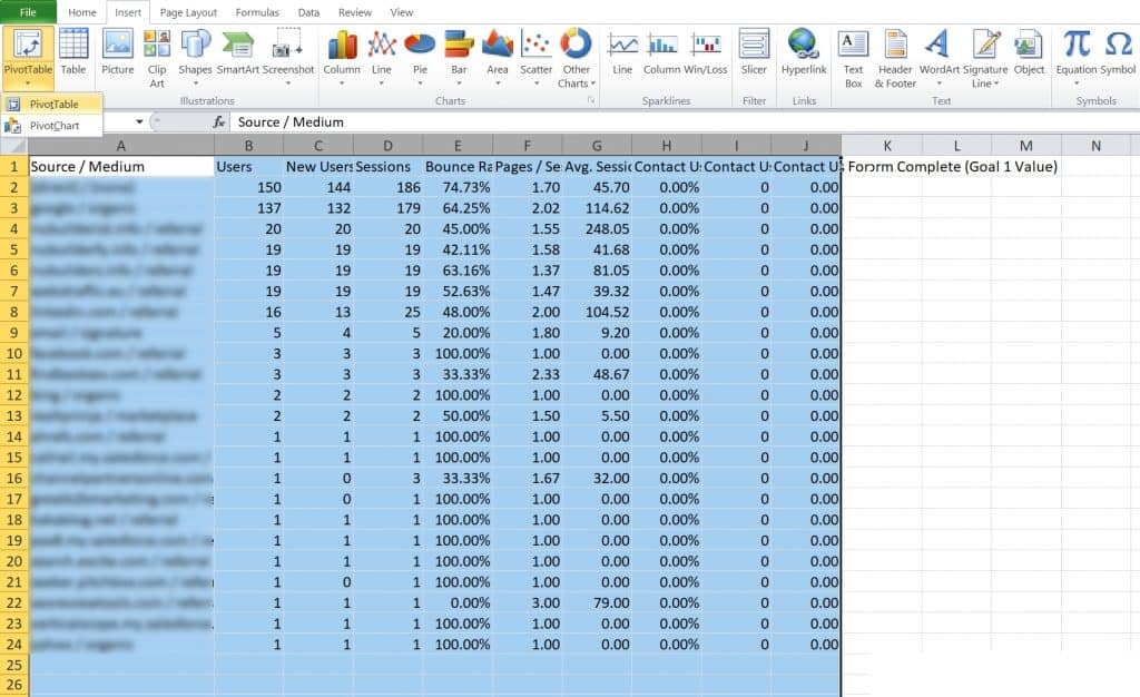
I like being able to customize graphs and tables the way I want them exactly. The easiest way to manipulate data in this way in Excel is with Pivot Tables. The main benefit of Pivot Tables is that you can drag-and-drop different data fields to quickly create graphs and tables. And pivot tables work well for small amounts of data or large databases. Let’s say you have to write a monthly report that features the same tables each month; it’s a real time saver to set-up a pivot table template that can spit out exactly what you need automatically. Below I will walk-through the process of creating a pivot table starting from a raw Google Analytics data export:
Navigate to ‘Acquisition’ -> ‘Source/Medium’.

These same techniques I’m going to demonstrate could be used for other reports within Google Analytics too.
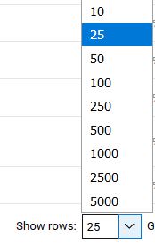
Along the bottom, click “Show rows:” and select 5000. This will ensure all traffic sources are exported.
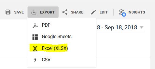
On the top ribbon, set the date range, then click “Export”, and choose “Excel (XLSX)”.
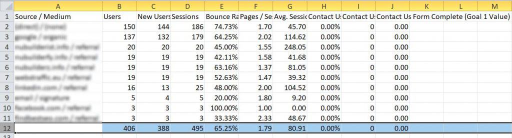
There’s three sheets: ‘Summary’, ‘Dataset1’, and ‘Dataset2’. The most useful data is in ‘Dataset1’, so that’s where we’ll be working.

At the very bottom of ‘Dataset1’, Google automatically includes a row of totals. Delete this entire totals row or it’ll throw off your numbers.
Select the whole table, Column ‘A’ through to ‘J’. Navigate to the ‘Insert’ tab, click ‘PivotTable’, and again click ‘PivotTable’.
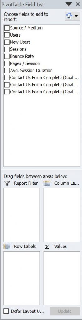
You should now see a blank PivotTable:

Now use the ‘PivotTable Field List’ to manipulate the data:
Try dragging the ‘Source / Medium’ field under ‘Row Labels’. Then click on all the metrics you’d like to include, and drag them under ‘Values’ .
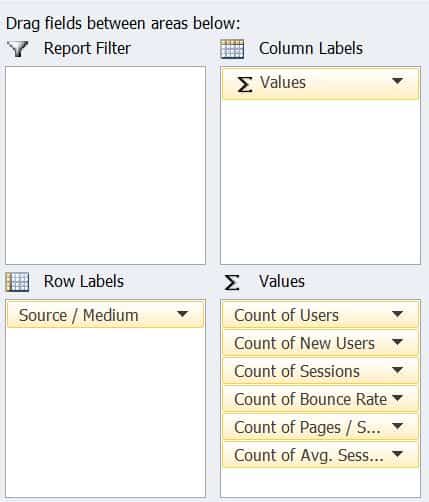
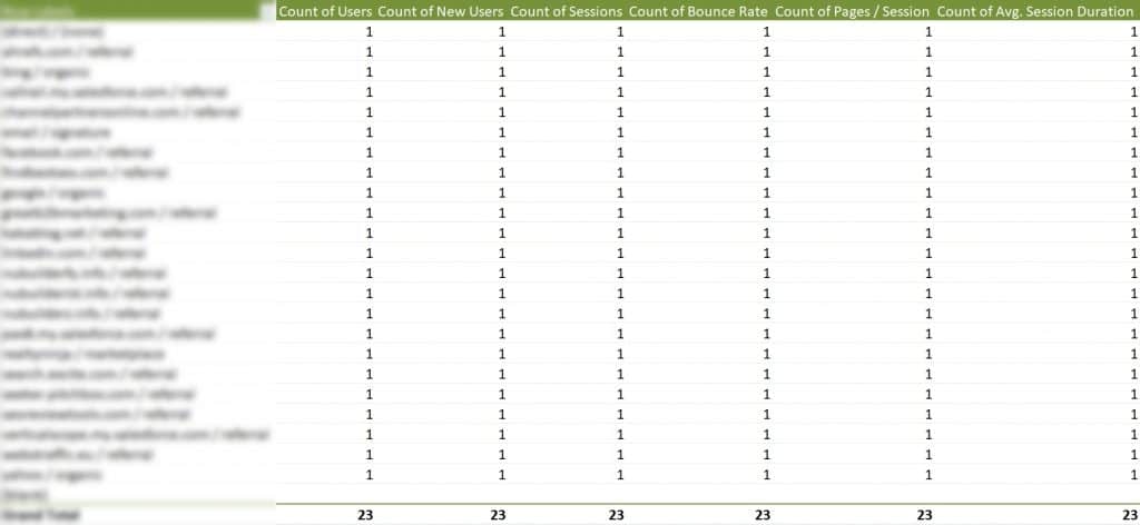
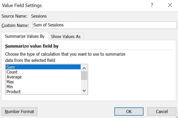
At this point, you should see a table that’s filled with 1’s. This is because all the metrics under ‘Values’ are defaulting to “Count”.
To get the correct totals, right click each item in ‘Values’, click ‘Value Field Settings’, and select ‘Sum’.
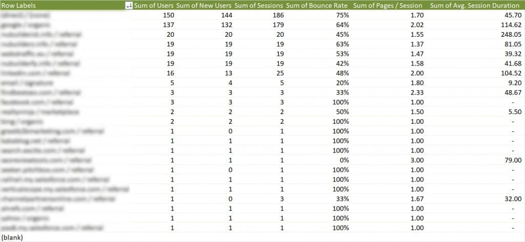
So now we have something that is starting to resemble a data table. It could use a little formatting help though.
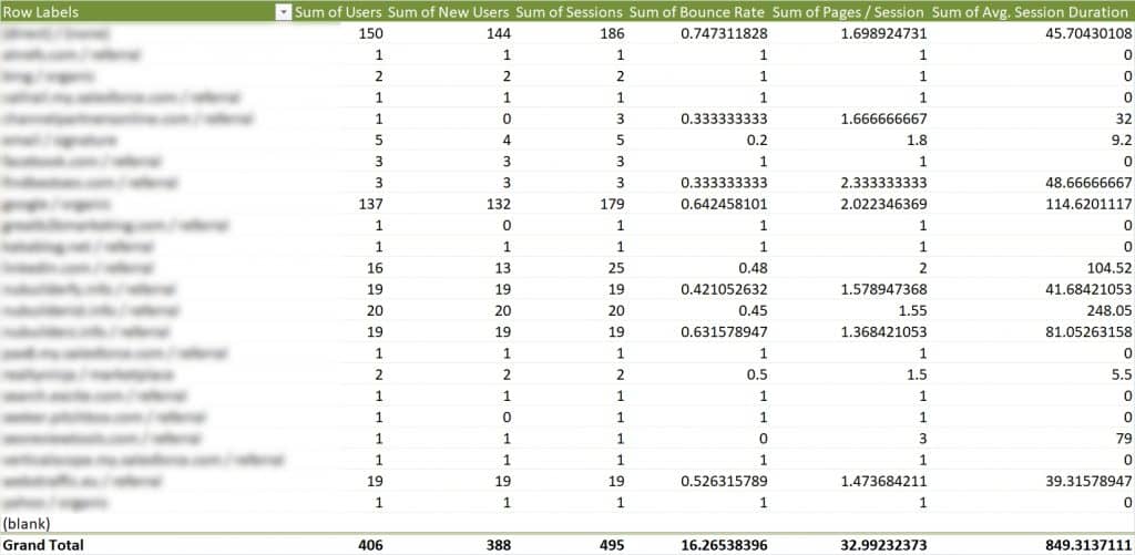
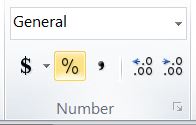
Click the top of the ‘Sum of Bounce Rate’ cell to select the whole column, then navigate to the Number tab to format as a percentage. Likewise, select the ‘Sum of Pages / Session’ and ‘Sum of Avg. Session Duration’ cells then format each column using ‘Comma Style’.
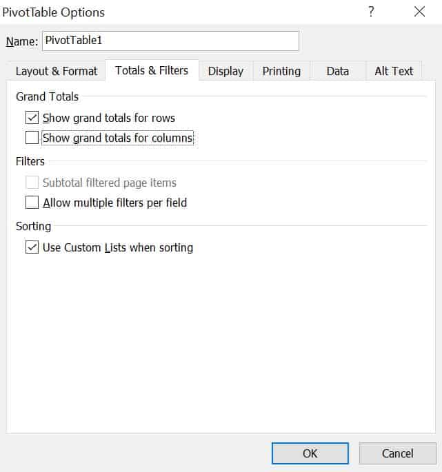
Next we’ll remove the automatically generated ‘Grand Total’, as it doesn’t make sense to calculate the total for metrics like ‘Avg. Session Duration’. Right click on the PivotTable, click ‘PivotTable Options’, click ‘Totals & Filters’, and deselect ‘Show grand totals for columns’.
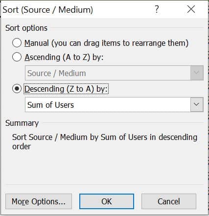
Now click on the drop down arrow next to ‘Row Labels’, click ‘More Sort Options’, then sort by ‘Descending…’, and select ‘Sum of Users’.
We have created a basic PivotTable utilizing Google Analytics data:
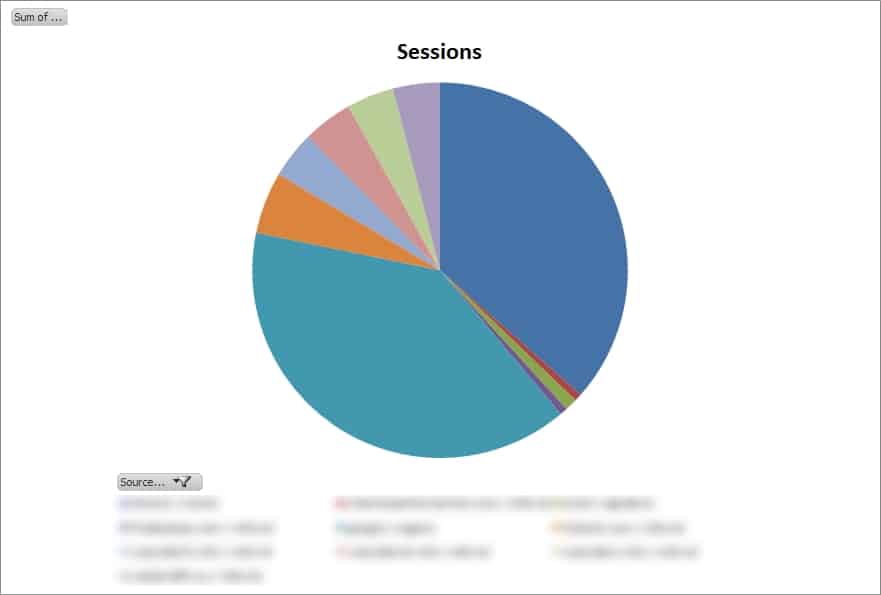
There are a lot of smaller things you can play with from here. You may want to filter out spam traffic sources and the “(blank)” row from ‘Row Labels’. You may want to rename the headings; if you try to rename “Sum of Users” to “Users”, you’ll get an error saying the field already exists, but if you add a space after, like “Users “, it will prevent this error. You may want to navigate to the ‘Design’ tab to see what formatting options you like. You may want to create additional PivotTables , or try creating some PivotCharts like the basic pie chart below.
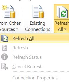
Once you have your PivotTable or PivotChart set-up to your liking, save it, and use it as a template for the future. The next time you want to run the same numbers, simply repeat steps 1-5 to export the Google Analytics data, then copy/paste the new data to replace the contents of the ‘Dataset1’ sheet, and click ‘Refresh All’ in the ‘Data’ tab. This will cause all PivotCharts and PivotTables drawing from ‘Dataset1’ to update instantly.
Once you get the hang of PivotTables, it becomes quick to set them up, polish them, and to make iterations. They really are a great source of time savings and consistency if you’re having to run the same reports regularly. And trust me, you’re going to need all the time savings you can muster once word gets out in the office about your newly found Excel skills.
Do you need help making sense of your marketing analytics? eBridge can help. Please contact us for more information.

As eBridge’s VP of Operations, Devin Rose brings marketing expertise and an entrepreneurial knack to the eBridge team. Devin holds a Bachelor of Commerce Degree from Royal Roads University and a Marketing Management Diploma from the British Columbia Institute of Technology.
Posted May 8, 2019
Categories: Advertising and Marketing General,
Marketing Analytics,
Search Engine Strategies (SEO & PPC),
Social Media Management
Tags: concatenate, Google analytics, how to, Marketing Analytics, microsoft excel, pivot tables, tracking links